Lösung von Teilaufgabe c) 2.: Unterschied zwischen den Versionen
Aus RMG-Wiki
(→Verwendung der Tangentialgleichung) |
(→Verwendung der Tangentengleichung) |
||
| (11 dazwischenliegende Versionen von einem Benutzer werden nicht angezeigt) | |||
| Zeile 2: | Zeile 2: | ||
| − | === Verwendung der | + | === Verwendung der Tangentengleichung === |
| + | Hier rate ich wieder zur Verwendung der Tangentengleichung.<br /> | ||
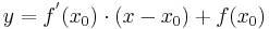
: <math>y = f^{'}( x_0)\cdot ( x - x_0 ) + f ( x_0 )</math><br /> | : <math>y = f^{'}( x_0)\cdot ( x - x_0 ) + f ( x_0 )</math><br /> | ||
| + | Zwar fehlen hier einige feste Werte, die man in die Gleichung einsetzen kann, doch diese hat man in allgemeiner Form durch die Funktion und die erste Ableitung gegeben.<br /> | ||
:<math> y = ( x_0 - a - 1 )\cdot ( -e^{a + 2 - x_0})\cdot ( x - x_0 ) + ( x_0 - a )\cdot e^{a + 2 - x_0})</math><br /> | :<math> y = ( x_0 - a - 1 )\cdot ( -e^{a + 2 - x_0})\cdot ( x - x_0 ) + ( x_0 - a )\cdot e^{a + 2 - x_0})</math><br /> | ||
| Zeile 27: | Zeile 29: | ||
:: <math>\Rightarrow ( x_0^{2} - 2\cdot x_0 - 2 ) = 0</math> | :: <math>\Rightarrow ( x_0^{2} - 2\cdot x_0 - 2 ) = 0</math> | ||
| − | + | ||
| + | Nun hat man als Lösung eine Quadratische Gleichung erhalten. <br />Diese löst man am besten mit Hilfe der Mitternachtsformel.<br /> | ||
Lösen quadratischer Gleichungen mit Hilfe der [http://de.wikipedia.org/wiki/Mitternachtsformel?title=Mitternachtsformel&redirect=no Mitternachtsformel] <math> x_{1,2} = \frac{-b\pm\sqrt{b^{2}-4\cdot a\cdot c}}{2a}</math> | Lösen quadratischer Gleichungen mit Hilfe der [http://de.wikipedia.org/wiki/Mitternachtsformel?title=Mitternachtsformel&redirect=no Mitternachtsformel] <math> x_{1,2} = \frac{-b\pm\sqrt{b^{2}-4\cdot a\cdot c}}{2a}</math> | ||
| Zeile 35: | Zeile 38: | ||
:: <math> = \frac{2\pm2\cdot\sqrt{3}}{2}= {1\pm\sqrt{3}}</math><br /> | :: <math> = \frac{2\pm2\cdot\sqrt{3}}{2}= {1\pm\sqrt{3}}</math><br /> | ||
| − | |||
| − | |||
: <math>\Rightarrow x_{1} = {1 + \sqrt{3}}</math><br /> | : <math>\Rightarrow x_{1} = {1 + \sqrt{3}}</math><br /> | ||
| Zeile 42: | Zeile 43: | ||
: <math>\Rightarrow x_{2} = {1 - \sqrt{3}}</math><br /> | : <math>\Rightarrow x_{2} = {1 - \sqrt{3}}</math><br /> | ||
| + | Die beiden nun erhaltenen x-Werte müssen nun nur noch in die Funktion eingesetzt werden.<br /> | ||
| − | + | [[Bild:Tangente_b1111.png|400px|right]] | |
: <math>f_a(x_1)=\;</math><br /> | : <math>f_a(x_1)=\;</math><br /> | ||
::: <math>= f_a(1 + \sqrt{3})\;</math> | ::: <math>= f_a(1 + \sqrt{3})\;</math> | ||
| Zeile 52: | Zeile 54: | ||
::: <math>\approx 2{,}601</math><br /> | ::: <math>\approx 2{,}601</math><br /> | ||
| − | + | :::: <math> \Rightarrow B_1(1 + \sqrt{3} / 2{,}601)</math> | |
| − | :::: | + | |
| − | + | ||
| Zeile 62: | Zeile 62: | ||
| − | [[Bild: | + | [[Bild:Tangente_b2222.png|400px|right]] |
: <math>f_a(x_2) =\;</math><br /> | : <math>f_a(x_2) =\;</math><br /> | ||
::: <math>= f_a(1 - \sqrt{3})\;</math> | ::: <math>= f_a(1 - \sqrt{3})\;</math> | ||
| Zeile 71: | Zeile 71: | ||
::: <math>\approx -310{,}164</math><br /> | ::: <math>\approx -310{,}164</math><br /> | ||
| − | + | :::: <math> \Rightarrow B_2(1 - \sqrt{3} / -310{,}164)</math> | |
| − | |||
| + | Nachdem beide Berührpunkte nun einzeln gezeigt worden sind, hier eine Grafik in der Beide gleichzeitig zu sehen sind. | ||
[[Bild:TANGENTE_b1b2.png|400px]] | [[Bild:TANGENTE_b1b2.png|400px]] | ||
Aktuelle Version vom 26. Januar 2010, 21:12 Uhr
Berechnung derjenigen Punkte, für welche die Tangente an den Graphen von f2 durch den Ursprung verläuft
Verwendung der Tangentengleichung
Hier rate ich wieder zur Verwendung der Tangentengleichung.
Zwar fehlen hier einige feste Werte, die man in die Gleichung einsetzen kann, doch diese hat man in allgemeiner Form durch die Funktion und die erste Ableitung gegeben.


Nun hat man als Lösung eine Quadratische Gleichung erhalten.
Diese löst man am besten mit Hilfe der Mitternachtsformel.
Lösen quadratischer Gleichungen mit Hilfe der Mitternachtsformel 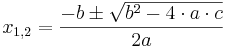

Die beiden nun erhaltenen x-Werte müssen nun nur noch in die Funktion eingesetzt werden.


Nachdem beide Berührpunkte nun einzeln gezeigt worden sind, hier eine Grafik in der Beide gleichzeitig zu sehen sind.
